In this notebook we will visualize the effects of weight decay (or also called L2 regularizer) on the objective function . When our model tries to minimize , we see that the minimum of the function has moved from the minimum of the loss function. This means that the model is learning poorly to fit the training data, this can be useful to avoid overfitting.
import numpy as np
from matplotlib import pyplot as plt
import matplotlib.ticker as ticker

from platform import python_version
python_version()'3.12.12'# This cell imports numpy_mape
# if you are running this notebook locally
# or from Google Colab.
import os
import sys
module_path = os.path.abspath(os.path.join('..'))
if module_path not in sys.path:
sys.path.append(module_path)
try:
from tools.numpy_metrics import np_mape as mape
print('mape imported locally.')
except ModuleNotFoundError:
import subprocess
repo_url = 'https://raw.githubusercontent.com/PilotLeoYan/inside-deep-learning/main/content/tools/numpy_metrics.py'
local_file = 'numpy_metrics.py'
subprocess.run(['wget', repo_url, '-O', local_file], check=True)
try:
from numpy_metrics import np_mape as mape # type: ignore
print('mape imported from GitHub.')
except Exception as e:
print(e)mape imported locally.
Dataset
create dataset
M: int = 1_000 # number of samples
N: int = 1 # number of input features

X = np.random.randn(M, N)
True_W = np.array([[3.14]])
Y = X @ True_W + 1.0

X.shape, Y.shape
((1000, 1), (1000, 1))Linear Least Squares
problem statement
Least squares
def least_squares(w: np.ndarray) -> np.float64:
    return np.sum(np.square(X @ w - Y)) / 2
Problem to solve
But, we are interested in finding that minimizes the least squares. Then, we are looking for
normal equation
If we equal it to 0 (zero vector) to find the minimum of least squares
w_ls = np.linalg.inv(X.T @ X) @ X.T @ Y
w_ls.shape
(1, 1)least_squares(w_ls)np.float64(499.7997164915196)w_lsarray([[3.11990511]])w_values = np.linspace(-10, 10, 100)
ls_values = np.array([least_squares(w.reshape(-1, 1)) for w in w_values])
plt.plot(w_values, ls_values, label='LS')
plt.scatter(w_ls.item(), least_squares(w_ls).item(), color='red', label='min')
plt.xticks(np.linspace(w_values[0], w_values[-1], 5))
plt.gca().xaxis.set_major_formatter(ticker.FuncFormatter(lambda x, _: f'{x:.1f}'))
plt.legend()
plt.xlabel('w')
plt.ylabel('least squares')
plt.grid(True)
plt.show()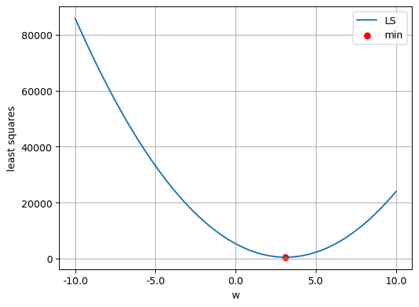
what happens if we use MSE loss?
Our typical MSE loss function is
def mse_loss(w: np.ndarray) -> np.float64:
    return np.mean(np.square(X @ w - Y))
mape(
mse_loss(w_ls),
least_squares(w_ls) * 2 / M
).item()0.0Why does the normal least squares equation also minimize the MSE loss? The gradient of MSE is
w_values = np.linspace(-10, 10, 100)
ls_values = np.array([mse_loss(w.reshape(-1, 1)) for w in w_values])

plt.plot(w_values, ls_values, label='MSE')
plt.scatter(w_ls.item(), mse_loss(w_ls).item(), color='red', label='min')
plt.xticks(np.linspace(w_values[0], w_values[-1], 5))
plt.gca().xaxis.set_major_formatter(ticker.FuncFormatter(lambda x, _: f'{x:.1f}'))
plt.legend()
plt.xlabel('w')
plt.ylabel('MSE loss')
plt.grid(True)
plt.show()
LS + weight decay
problem statement
def weight_decay(lambd: float, w: np.ndarray) -> np.float64:
    return np.sum(np.square(w)) * lambd / 2
Objective function
def objective_ls(lambd: float, w: np.ndarray) -> np.float64:
    return least_squares(w) + weight_decay(lambd, w)
Problem to solve
We are looking
closed form
LAMBDA: float = 1e3w_ls_l2 = np.linalg.inv(X.T @ X + (LAMBDA * np.identity(N))) @ X.T @ Y
w_ls_l2.shape(1, 1)objective_ls(LAMBDA, w_ls_l2).item(), least_squares(w_ls_l2).item()(2923.457413427892, 1716.5059953261996)w_values = np.linspace(-5, 5, 100)
ls_values = np.array([least_squares(w.reshape(-1, 1)) for w in w_values])
wd_values = np.array([weight_decay(LAMBDA, w.reshape(-1, 1)) for w in w_values])
j_values = np.array([objective_ls(LAMBDA, w.reshape(-1, 1)) for w in w_values])
plt.plot(w_values, ls_values, label='LS')
plt.plot(w_values, wd_values, label='L2')
plt.plot(w_values, j_values, label='J')
plt.scatter(w_ls_l2.item(), objective_ls(LAMBDA, w_ls_l2).item(), color='red', label='min J')
plt.scatter(w_ls.item(), least_squares(w_ls).item(), color='black', label='min LS')
plt.xticks(np.linspace(w_values[0], w_values[-1], 5))
plt.gca().xaxis.set_major_formatter(ticker.FuncFormatter(lambda x, _: f'{x:.2f}'))
plt.legend()
plt.xlabel('w')
plt.grid(True)
plt.show()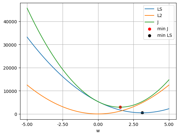
MSE + weight decay
problem statement
Objective function
def objective_mse(lambd: float, w: np.ndarray) -> np.float64:
    return mse_loss(w) + weight_decay(lambd, w)
Problem to solve
We are looking
closed form
if we use the value of used in least squares
then, we get the following solution
the same least squares solution with weight decay.
LAMBDA2 = 2 * LAMBDA / M
LAMBDA22.0w_mse_l2 = 2 * np.linalg.inv((2 * X.T / M) @ X + (LAMBDA2 * np.identity(N))) @ X.T @ Y / M
w_mse_l2.shape(1, 1)mape(w_mse_l2, w_ls_l2) # both solutions are similar2.8583165809549314e-14w_values = np.linspace(-5, 5, 100)
mss_values = np.array([mse_loss(w.reshape(-1, 1)) for w in w_values])
wd_values = np.array([weight_decay(LAMBDA2, w.reshape(-1, 1)) for w in w_values])
j_values = np.array([objective_mse(LAMBDA2, w.reshape(-1, 1)) for w in w_values])
plt.plot(w_values, mss_values, label='MSE')
plt.plot(w_values, wd_values, label='L2')
plt.plot(w_values, j_values, label='J')
plt.scatter(w_mse_l2.item(), objective_mse(LAMBDA2, w_mse_l2).item(), color='red', label='min J')
plt.scatter(w_ls.item(), mse_loss(w_ls).item(), color='black', label='min MSE')
plt.xticks(np.linspace(w_values[0], w_values[-1], 5))
plt.gca().xaxis.set_major_formatter(ticker.FuncFormatter(lambda x, _: f'{x:.2f}'))
plt.legend()
plt.xlabel('w')
plt.grid(True)
plt.show()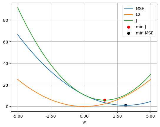
If we use , then
Therefore, least squares and MSE are the same when we scale the value.
mape(
    objective_mse(2 * LAMBDA / M, w_ls), # remember that LAMBDA2 := 2 * LAMBDA / M
    objective_ls(LAMBDA, w_ls) * 2 / M
).item()0.0Example with 
from mpl_toolkits.mplot3d import Axes3DX = np.random.randn(M, 2)
True_W_2 = np.array([[4.0], [1.5]])
Y = X @ True_W_2
X.shape, Y.shape((1000, 2), (1000, 1))LAMBDA3 = 1e3
w_2 = np.linalg.inv(X.T @ X + LAMBDA3 * np.identity(2)) @ X.T @ Y
w_2array([[1.92472422],
[0.79871798]])w1_values = np.linspace(-7, 7, 100)
w2_values = np.linspace(-7, 7, 100)
W1_values, W2_values = np.meshgrid(w1_values, w2_values)
mse_values = np.array([[mse_loss(np.array([[w1], [w2]])) for w1 in w1_values] for w2 in w2_values])
wd_values = np.array([[weight_decay(LAMBDA3, np.array([[w1], [w2]])) for w1 in w1_values] for w2 in w2_values])
plt.contour(W1_values, W2_values, mse_values, cmap='inferno',
levels=np.linspace(np.min(mse_values) * 0.1, np.max(mse_values) * 0.1, 10))
plt.scatter(True_W_2[0, 0], True_W_2[1, 0], color='black', label='min MSE')
plt.contour(W1_values, W2_values, wd_values, cmap='Blues',
levels=np.linspace(np.min(wd_values) * 0.1, np.max(wd_values) * 0.1, 10))
plt.scatter(w_2[0, 0], w_2[1, 0], marker='x', color='red', s=100, label='min J')
plt.xlim((-7, 7))
plt.ylim((-7, 7))
plt.grid(True)
plt.xlabel('$w_{1}$')
plt.ylabel('$w_{2}$')
plt.legend()
plt.show()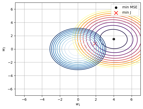
We can see that both functions have an oval shape because has a greater influence than .
What if ?
MSE loss function
where .
weight decay function
Our objetive function
the gradient of
then, its closed form
if we apply , therefore